History of Baruch Exhibit: Part 4, Item 4.8

DECISION THEORY AND ECONOMETRICS

The empirical evidence tends to suggest that a public lecture may be characterized as an occasion on which a speaker communicates effectively with a very small fraction of his audience for a very small fraction of the time. I do not advance this definition in any arrogant fashion, for I realize only too well that it is possible to miss a target in many directions, and indeed a dull parade of vacuous platitudes that should not be repeated outside of kindergarten is perhaps an even worse form of non-communication than a lecture which shoots off into outer space with a dazzling display of pyrotechnics. So I will try to steer a middle course between these twin dangers.-

For my subject I have chosen "Decision Theory and Econometrics," and I should like to try to cover three main points. The first is a presentation of a bird's eye view of the general field of decision theory. This will give us a perspective from which to see the section of that field in which econometrics has a function or role to play. Second, I want to look critically at some of the main econometric models that have been constructed with a view to helping the decision-making process. Third, I will touch upon the ways in which econometric models may be incorporated with varying degrees of formality into decision-making processes. To keep the subject manageable I will be looking only at macroeconometric models in which the relevant decisions are those of government for purposes of economic policy and control. This is the most glamorous but at the same time almost certainly the most difficult area for econometric work, and it does mean that we will not be discussing any of the micro or sectional areas in which a great deal of valuable and reasonably successful econometric work has been done.-

On the principle that anyone who comes to a public lecture deserves at least one moment of pleasure, let me begin on a lighthearted note.-

A recent cartoon shows a holiday-maker on a beach. On the left his wife is sinking beneath the waves with a last despairing cry of "Help!" On the right his drinking companions proclaim the joyful news "The pubs are open!" The caption reads "Decisions, decisions, always decisions". Rather unwittingly this piece of nonsense gives a fairly accurate description of the dilemma that faced Harold Wilson when the Labour Government took office in the. United Kingdom in late 1964. On the one hand, sterling was being battered by successive waves of speculative attack. On the other hand, it must have seemed very inviting, metaphorically speaking of course, to go into the pub and stand treat all round, distributing three percent mortgages, increased old age pensions and all the rest of the promised election bonanza.

In each case the decision problem is almost identical. If we distribute the economic and social benefits first, is sterling inevitably doomed? If we defend sterling can we distribute the social dividend later and, if so, how much later and to what extent? As a matter of record the only social dividend distributed in the early months of the Government was a very substantial increase in the salaries of Members of Parliament. A decision to increase old age pensions was taken-with a specified delay in implementation, and three percent mortgages remain to this day a figment of George Brown's overstimulated imagination. The holiday-maker, one might think, has no real problem at all. He simply rescues his wife and then retires with honour to the saloon bar. This, however, implies two crucial assumptions, one concerning his utility function, that is, his objectives and the values he places upon them, and the other his technical prowess as a life-saver. In other words, the suggested decision is certainly optimal if he doesn't wish his wife to drown and if he is certain to be able to rescue her and thus live to return to the delights of the bar. Suppose, however, that with his utility function unchanged, we allow uncertainty about his life-saving prowess to creep into the picture. If he plunges in to the rescue, there are now several possible results: he may perhaps drown along with his wife; he may fail to rescue her, but survive himself; he may perish himself while his wife is rescued by a heroic passer-by or finally he and his wife may both survive. The situation may become still more complicated if, in the event of his own survival, there is the additional possibility that he may have swallowed so much sea-water that his imminent enjoyment of alcohol is likely to be delayed or even seriously impaired. The problem can easily become so complicated that the holiday-maker would be well advised to give some thought to it before going on holiday. He might even decide not to risk moving from home at all.

This imaginary problem introduces the basic elements of real decision problems. There is, first of all, the set of possible decisions or actions; there is secondly the set of possible outcomes or results and there is thirdly the network of relationships connecting decisions and outcomes. One additional feature of many real-life situations is that some decision problems occur again and again. One would not like to think of our holiday-maker facing the same problem year after year, with the same wife or with a succession of wives, depending upon his decisions in previous years. However, decisions about taxes, monetary policy and the like have to be taken at frequent intervals by governments; decisions about production, pricing, advertising and so on have to be taken frequently by business firms and similarly for decisions about earning, spending and saving by consumers. In sequential decisionsas distinct from single decisions-the extent to which one attempts to allow for the possible effects of present decisions on future decisions is an added complication, and this in turn depends upon the time horizon which the decision-maker takes into consideration.

In recent years economists, operational researchers, political scientists and others have devoted an increasing amount of time and effort to the study and analysis of decision problems, mainly in the fields of business and government. The main feature of their efforts is an intensive use of logical, mathematical, and statistical methods in an attempt to obtain a fairly realistic and operational specification of a problem in order to search for optimal solutions in areas which hitherto have had to be treated mainly on the basis of hunch and intuition. These developments have often depended crucially on the availability of large scale modern computing equipment. In order to obtain a bird's-eye view of these developments, let us return for a moment to the basic elements in a decision problem that have already been mentioned and sketch them in Figure I.

For our purposes we may classify decision problems by the nature of the network of relationships connecting actions and outcomes. Networks can range all the way from simple, direct and certain connections between specific actions and specific results to vast, complicated, very uncertain and even possibly unknowable networks.

In the instance of a simple network, actions can be joined directly to outcomes by passing straight lines one-to-one through the network box. For example, in choosing a computer system, or a university to work at, or a wife to live with, you make your choice from the list of available options and you get the one you have chosen. Making the actual choice, however, can be agonizingly difficult since the outcome is often multi- dimensional. As shown in Figure II, action gives the outcome , which has dimensions and the index i ranges over the set of available actions. Here the techniques of cost-benefit analysis come into play since they are concerned with bringing into a single total reckoning the "value," in some sense, of one outcome compared with another.

To give a homely illustration the relevant dimensions of a university might be the salary offered, the chairman, one's colleagues, the computer set-up, the quality of the students, the distance to the nearest golf course, climate, etc. I have not listed these in any priority order, and climate should not necessarily be put at the bottom of the list. The chairman of at least one well known department writes pleasant and frequent letters to various people describing the delights of his campus by quoting the average winter temperature and the average summer temperature, but he never says anything about the deviations from the average. This may reflect deficiencies in his statistical training or it may, of course, be a deliberate withholding of information.

On the other hand, an outcome may be adequately measured by a single variable such as cost or profit but the action may be multidimensional, as in the determination of product-mix in a multiproduct plant. In this instance, which is sketched in Figure III, optimal decisions may be studied by means of the calculus or by the methods of linear or nonlinear programming, depending on the structure of the problem. The extension from static to dynamic problems covering several time periods may often be handled by the same methods, though more realistic formulations almost certainly require the use of dynamic programming methods.

Thus far we have been postulating simple and direct connections between actions and outcomes. Next we must allow uncertainty to creep into the picture so that the actual outcome corresponding to a given action is one and only one of some specified set of outcomes.

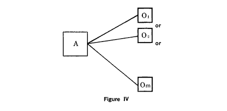
For example, we set a production rate (A), but the terminal inventory () depends upon demand, which is a stochastic variable that we cannot predict precisely. This instance characterizes a range of problems to which the techniques of statistical decision theory are being increasingly applied, the emphasis being placed on the evaluation of utilities, a priori probabilities for various outcomes, the possible incorporation of sample information to revise and update these probabilities and the taking of action to maximize expected utilities.

We see then that in the instance of simple network problems we have major techniques like cost-benefit analysis, mathematical programming and statistical decision theory that may be brought to our aid. Although each of these subjects is now an intellectual specialization in its own right, you may make some progress if you can select the right specialist for your problem.

When we turn to large economic systems, however, especially to the national economy as viewed by a government or a particular sector of it which is of direct concern to a business firm, we immediately find ourselves in much more difficult territory. The first source of difficulty is that the network problem is now immeasurably more complicated. So far as we know the values assumed by economic variables are determined by the simultaneous interaction of a large number of relationships: most variables play a role in more than one relation of the system; the relations are not simple, exact ones but are subject to random fluctuations, just as if a given degree of pressure on the brake pedal of a car cannot always be relied upon to produce a specific reduction in speed, but sometimes might produce one reduction and at others another. Finally the relations themselves may change as time passes, just as if someone had changed the whole system of linkages connecting the brake pedal to the brake drums. The second source of difficulty in the management of economic affairs is that both actions and outcomes are multi-dimensional. We often want to affect a number of variables and we need to move a number of controls to do so.

Turning now to the network problem in economics we may approach it in a number of ways.

The simplest approach of all is to say there are no laws of economic dynamics, that each economic event is unique, influenced by such a myriad of factors that to all intents and purposes the economic system can be regarded as a gigantic lottery, unpredictable and uncontrollable. Naturally, this is a proposition fiercely resisted by economists and politicians alike, since its acceptance would destroy the profession of the former and seriously circumscribe the activities of the latter. Nor would it give any comfort in the board rooms, for why should we pay directors fat salaries to make decisions if we would do just as well by asking a computer to generate a few random numbers!

The next level of approach is to recognize that a given economic system is a very complex one, so complex indeed that no feasible model of the system can be formulated explicitly. Instead, great emphasis is placed on notions of intuitive judgment, hunch, feeling for and assessment of the situation. Unfortunately, it is not clear how much judgment is to be acquired and still less clear how it is to be taught or communicated persuasively to someone whose judgment leads him to forecast a different outcome. Nonetheless, many economic commentators and advisers have operated (and still do operate) in this way, their pronouncements often making up in vigor for what they lack in analytical rigor.

A third approach is to build a theory or model, however simplified and approximate, of the relationships which are thought to determine the values assumed by the economic variables under study. The basic assumptions incorporated in the model may be derived from judgments formed about particular aspects of the economic system or they may be based on simple principles or rational behavior, but now at least the assumptions are made explicitly and the working out of the theory will display the full implications of the assumptions made. In most countries, this is the end of the line, and it is quite customary for the economic theorist to make a swift transition from manipulating his models of economic man to advising the Chancellor of the Exchequer on suitable taxation to impose on the business man. In such situations economic theories survive and may have a political impact, not necessarily on the basis of their relevance to the world with which they purport to deal, but rather on the debating skill, the academic pedigree, or the political and social connections of the theorist.

There are several difficulties in a purely theoretical approach. First of all, the type of theoretical model that can be handled analytically and manipulated by a single brain rather than by a large computer may be too simple and too small to give an adequate representation of a complex system. Secondly, one man's theory, even if sufficiently complex, is not necessarily a correct description of the system. What about the next man's theory? How do we choose between them? Thirdly, even if the theoretical specification of the model is reasonably good, numerical estimates of the coefficients in the relationships are often required if any practical use is to be made of the theory. For in an interrelated system the net effect of changing any decision variable will depend in a fairly complicated fashion on many coefficients from various equations in the model. Even strong a priori convictions about the signs of these coefficients will not usually give unambiguous indications about the sign, much less the amount, or the net effect in question.

It is to help with these difficulties that econometrics has developed as a practical subject. It is essentially concerned with replacing the Greek letters which represent the parameters of a theoretical model with numerical coefficients obtained by processing data from an economic system. In principle, econometric investigations can then afford us two important advantages. First, they sometimes enable us to discriminate between economic theories, to prefer one to another as being more consistent with the data. A second is the making of numerical predictions. All predictions are subject to the condition that an appropriate model has been used and that the relationships of the model are stable and will continue to hold in the prediction period. Even with these provisos there are two elements of uncertainty which cannot be eliminated from such predictions. The first is due to the effects of exogenous variables beyond the control of the policy maker; effects which cannot usually be accurately forecast by the model builder. The second is due to the stochastic nature of all economic relationships. Although economic theorists usually work with exact functional relationships between variables, no data are ever observed to yield such functions. Thus the econometrician's statistical technique depends crucially upon the insertion of a stochastic error term into his fitted relationships. The exact value of this error term on any future occasion cannot be known, but probability statements can be made about the limits within which it may lie. Julian Huxley once described God as "a personified symbol for man's residual ignorance," and the stochastic error term plays a similar role in the econometrician's scheme of things. We know it is there. We are not at all sure of what it is like, nor can we observe it. Yet for practical purposes we must make certain assumptions about it. It is, in a sense, a measure of our residual, and possibly irreducible ignorance about the economic system.

Before using an econometric model, however, we must validate the model: we must ask whether the model is sufficiently good to be put to use or whether it must be modified and further improved. In practice one employs a combination of tests in judging the validity of an econometric model, but I am going to concentrate here on only two tests. The first is the forecasting performance of the model outside the sample period that has been used in fitting the relationships and the second (and subsidiary) test is the stability of the model's coefficients when re-estimated with some additional data.

The Oxford Econometric Model of the United Kingdom-19481956 (Tables 1 & II)

The Oxford model consists of thirty-seven equations applied to U. K. quarterly data for the years 1948 to 1956. The choice of a quarter as the basic time unit emphasizes the fact that the central objective of the model was the description and analysis of short-run movements of the economic system. This proved most difficult to achieve because of limitations of both theory and data. Indeed the authors had to "invent" quite a lot of theory and some of the data as well. Comparative statics and long-run growth theory are no help in formulating equations to tell us where we will be next quarter in relation to our current position in this one,

and conventional trade-cycle theory is not very explicit about the basic time period to which the analysis is supposed to relate. The data position at that time was disastrously bad in the U. K. As there were no quarterly national income data, the model had to be built around the U. K. Production Index, and as several other series were not available on a quarterly basis, quarterly "estimates" had to be made by the authors.

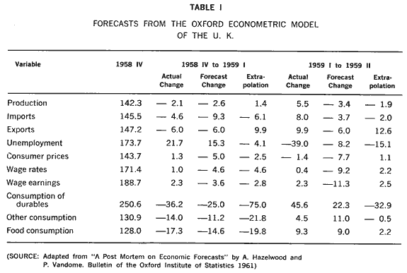
Table I shows two sets of forecasts from the Oxford model for quarters outside the period to which the model was fitted.

As Figure V shows, the accuracy of a forecast depends on two factors: the accuracy of the values inserted by the forecaster for the predetermined variables and the correctness of the structure of the model. Since we are interested here in the second factor only, we must purge the forecasts of any errors of the first kind. This can be done after a sufficient lapse of time and the result is shown in Table I in the columns headed "Extrapolation." The comparison of the extrapolation with the actual change is then an indication of the correctness and the stability of the model structure. Unfortunately, most macro-econometric predictions to date have been given in the form of point predictions and not in the form of a range of possible values, so we have to use judgment unaided by statistical tests in comparing these figures.

In this case, however, the judgment is reasonably clear. Comparing extrapolation with actual change from 1958/4 to 1959/1, we observe that six variables out of ten have the direction of change incorrectly predicted: production and exports were expected to rise, but they fell; unemployment was expected to fall but it actually rose substantially; and falls in consumer prices and wage rates were incorrectly predicted. Strangely enough, the forecast changes based on incorrect values of the predetermined variables are much better than the extrapolations-a striking case of two wrongs making a right. The direction of change is now incorrect in only three instances out of ten, and substantial improvements appear in production, exports, unemployment, and the consumption of durables. Comparing actual change and extrapolation for the next quarter, we see that the direction of change is incorrectly predicted five times out of ten. The forecast changes fare differently but no worse, with five signs wrong. Counting signs, however, is possibly too severe a way of looking at this model, for the actual changes are very small for 3 or 4 of the variables-less than 1 or 2 percent-and thus extremely difficult to predict. However, the predictions are still poor for production, unemployment and durable consumption.

Table II shows the effect on the estimated parameters of the model when two additional years of data were added to the sample. The three main sources of variation in these coefficients are sampling error, incorrect specifications of the model and changes in structure. Although there are no objective criteria of what constitutes "significant" changes in coefficients if these were due to sampling variations alone, there are some fairly large changes. One-half of the coefficients vary by less than 25 percent; just over three-quarters of all the estimates vary from one-half to double their initial value; and three fall to less than one-tenth of their initial value. In the equation for consumption of services in the original model, the only significant variable was wage income, with a coefficient eighteen times its standard error, yet the addition of two further years of data renders its coefficient insignificant.

Clearly' this set of 37 equations did not adequately describe the functioning of the British economy in those years. Would a model of 3 equations or 7 equations have done better or should there have been 370? Let us see how other models have fared.

The Klein- Goldberger Model of the U.S.A.-1929-1952 (Table III)

This is a system of 21 equations fitted to annual data for the U.S.A. for the period 1929-1952, omitting the war years. Table III shows the forecasting performance of this model for the first three years beyond the sample period. These are ex ante forecasts in the sense that only estimated values of the predetermined variables have been used. The forecast for 1953 was prepared with data available at March 1953 only; that for 1954 was prepared in

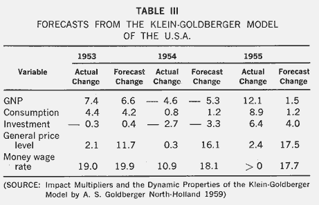
November 1953; and, similarly, that for 1955 was prepared in November 1954, but with the use as well of such independent information as surveys of investment plans. It is interesting to note that the model correctly forecast the down-turn in GNP in 1954, and also a rather subtle development, a slight rise in consumption in that year. It also forecast an upturn in 1955, but seriously under-estimated the extent of that up-turn. However, the last two lines of the table show the money side of the model to be deficient. Price movements are consistently over-estimated, and so is the wage change in two of the three years. Further detailed work by Goldberger in his excellent book on Impact Multipliers showed that the investment function was one of the weakest relations in the model and that the errors in forecasting GNP were highly correlated with errors in forecasting investment. He concluded:

"Mechanical use of an econometric model to predict GNP is inadequate. Careful study of recent residuals, combined with a resort to supplementary information such as that contained in surveys of investment intentions, can result in improved forecasting success."

Suits' (Michigan) Models

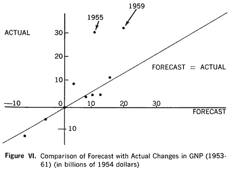
Goldberger's advice has been consistently followed by Suits and his colleagues at Michigan in their annual forecasts. Figure VI shows their record in forecasting changes in GNP for the years 1953-1961. No points lie in the second and fourth quadrants, that is, the directions of all changes were correctly forecast. The recessions of 1954 and 1958 were correctly predicted, though in each instance the extent of the recovery was under-predicted. Suits claims most success for his pessimistic forecast for 1960, made in November 1959, at the height of business optimism: "It proved to be more exact than any other forecast placed on record in advance."

Klein-Shinkai Econometric Model of Japan

Table IV shows the percentage errors for some basic variables in the Klein-Shinkai model of Japan. This is an annual model of 22 equations taking the years 1930-1936, 1951-1958 as a sample period but allowing for a structural shift in each equation between the prewar and postwar years. These errors are remarkably large, and in each instance, they are larger the further we go from the last year

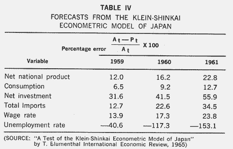
of the sample period. The author of this article concludes a survey of the forecasts of 18 variables:

"Only 4 out of 18 variables have an absolute error of less than 10 percent and only 7 have an absolute error of less than 20 percent in all 3 years. The worst projections, with an absolute error of more than 30 percent in each year are those for investment and unemployment. In 54 projections, 43 have lower values than the actual ones, indicating the under-estimating characteristic of the model." These projections are based on the true values of the predetermined variables, so that they are a direct indication of errors in the structure of the mode.

Macroeconomic Forecasts for the Netherlands

In the econometric world, the Netherlands is outstanding in two respects. The first is that for most of the post-war period the

Dutch have had an annual econometric model which is subject more or less to constant revision. The second is that the model is an official one, constructed at the Central Planning Bureau and used for making forecasts and analyzing possible policy moves.

Theil has carried out a very comprehensive analysis of the forecasting record of the Dutch model for 21 basic variables for the 10- period, 1953-1962. Table V shows that the models had a bias towards under-estimation of actual changes. Of the turning point

errors, there were 41 turning point forecasts of which 24 materialized and 17 did not. Of the 32 observed turning points, 24 were correctly predicted and 8 were not predicted.

Table VI shows some descriptive measures for selected variables. The letter r denotes the correlation between predicted change and actual change, and remembering that we are dealing with changes and not levels, we observe that most of the r's are quite good. There is, however, a fairly low correlation between predicted change and actual change for investment, and a negative one for exports. The meaning of the U coefficients may be seen as follows:

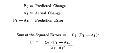
If there were no prediction errors at all, then would be zero. If one acted as a naive forecaster and said, "Next year will be the same as this year," i.e., = 0, then for such a forecaster = 1.

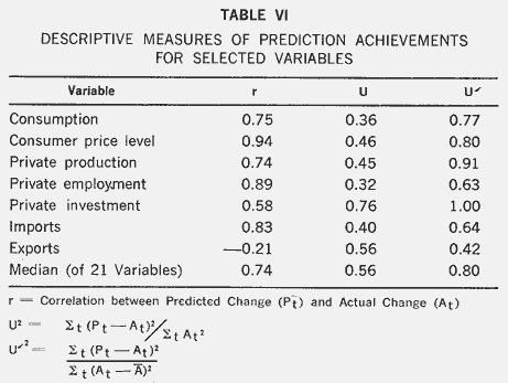
A less than one thus indicates a better performance than this naive forecast. However, U is too soft a comparison, for most economic variables increase with time, so that our naive forecaster would really be too naive. If he were smarter, he might take a pretty good estimate of the average rate of change () over the ten-year period and use this as his forecast every year. His squared

erros would then be

Thus , is defined from

As can be seen from Table VI, is greater than U. Exports have a U1 in excess of unity, so that a consistent prediction of would have been better than the model for this variable. For all 21 variables, however, the median value of is 0.80, and two-thirds have a less than 1, so that on average the are superior to the ., is almost certainly too severe a criterion for judging the model forecasts since the naive forecaster could not possibly know A accurately in advance. A recent article by C. A. Sims in the Review of Economics and Statistics (May 1967) replaces by simple trend projections of past observed changes. Only 2 of 22 variables now show aU value greater than unity for the period 19531963, and the average figure is 0.7.

The forecasts reported in Tables V and VI are genuine forecasts made ahead of time with imperfect knowledge of the predetermined variables. Table VII contains a comparison of these with conditional forecasts in which the true values of the predetermined variables

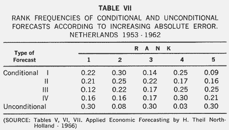
have been used. The various conditional forecasts (i) to (iv) depend on whether the wage rate and/or exports have been taken to be endogenous or exogenous. In (i), both have been taken as exogenous and in (iv) both are endogenous. We then have five forecasts for any variable for any year. These can be ranked from 1 to 5 by comparison with the actual change. Table VII shows the frequencies of those ranks. The unconditional forecasts occupy the worst position (fifth rank) more often than any other kind of forecast. However, the unconditional forecasts also have the greatest frequency in the first rank. Theil attributes this result to the forecaster's applying "amendments to the outcomes of the model computations in the light of extraneous information or common sense"-the Dutch, version of the flexible Michigan use of econometric models.

Table VIII is inserted as an interesting curiosity obtained from a recent article, as it is not often that people make direct comparisons of various econometric models for the same economy. This comparison focuses on the government expenditure multiplier only. The models differ in size (that is in the number of equations), specification, sample-time period, and basic unit-time period (annual or quarterly). The multiplier values come out fairly close for the annual models, but they are much higher for the quarterly model, though

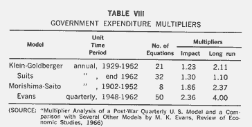
the author has averaged his quarterly multipliers in an attempt to approximate the yearly multiplier.

The Brookings Econometric Model of the U.S.A.

Table IX relates to an entirely different exercise. The Brookings Model of the U.S.A. differs from all previous macro-econometric models in several important respects. The first is size-400 or so equations rather than 20, 30, or 40. The second is in a method of construction. It utilizes an intellectual division of labor, with specialists working on the equations for various sectors rather than a single master-mind specifying the whole structure. The third feature is a consequence of the first two, namely much greater disaggregation. This is especially true of the investment and money sectors of the model. The fourth feature is a much more systematic attempt to get a good specification of the wage-price nexus and of the integration of real and money flows in the economy. The fifth is the integration of input-output analysis into the system.

One disadvantage of great size, however, is the time needed to compute all the equations, fit them together, and carry out manipulations of the model. The model was fitted to quarterly data for 1949-1960, the first full account being published in 196.5. It is impossible to say yet whether the model represents a substantial advance over its much smaller competitors. No comprehensive forecasting tests of the model have yet been published. The selections shown in Table IX come from an unpublished manuscript dispatched to the printers only last month. A denotes actual changes, denotes a series of 10 quarterly predictions based on the initial conditions of the second quarter of 1960, and a series of 8 quarterly predictions based on initial conditions at the fourth quarter of 1960. These pre-

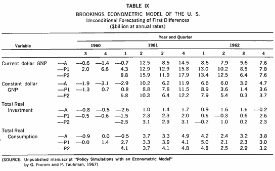
dictions have been obtained from a "reduced" version of the model consisting of about 180 equations.

Looking at the 8-quarter solution first of all, we note that the model fails to predict the decline in real GNP in the first quarter of 1961, but that the predicted rise from that period to the end of 1962 is not much less than the actual rise ($46.2 billion against $48.8 billion, or an error of about 5 % in the cumulated total over 7 quarters). For current dollar GNP the model fairly consistently overestimates the actual changes. For the same 7 quarters the cumulated actual change is $65.2 billion and the cumulated model change $85.6 billion, an overprediction of about 30 percent. Since the current value is derived as the product of a real value and a price index this suggests that the price equations in the model are overpredicting. Was this a structural break in the early years of the Kennedy era, or were the price equations in the model mis-specified for the whole of the sample period? As these first trial runs of the model appear, it seems clear that a fairly heavy program of revision and up-dating of the model lies ahead of the team at the Brookings Institution, and indeed much of this work is already under way.

On real GNP the 10 quarter solution does give some indication of the slight recession. On real investment both solutions indicate the recession and then tend to overpredict subsequent increases. On total real consumption neither solution does well on the early quarters, but both mirror movements very closely for the remaining 7 quarters. It must be emphasized, however, that the builders of this model still regard it as being in preliminary form, with a great deal of testing and re-estimation to be done.

Outstanding Questions

We have done enough to see that one can construct good econometric models or less good econometric models. It is clear that the economy does not yield up its secrets easily-either to the introspective theorist smoking a pipe in his study and gazing out at the college lawn or to the first econometrician who comes along with his raft of regression equations. On the econometric side, the outstanding questions seem to me to be mainly various aspects of the aggregation problem.

1) Aggregation over time. It seems a reasonable judgment that thus far the annual models have a better performance than the quarterly ones. Is the stochastic element relatively greater for the shorter time period? Are the problems of specifying lag structure and other features more intractable? Where should the balance of research-effort be put-into quarterly models or annual models?

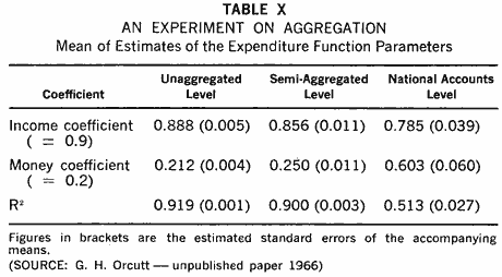
2) Aggregation over sectors and groups. The Brookings model, compared with previous macro-models, is an example of disaggregating from the top down. The gospel according to Guy Orcutt, a prophet crying not in the wilderness but in the Middle West, is that we should aggregate from the bottom up. In principle, when one thinks of the possible heterogeneity of the behavior of different groups and sectors he is right. Even with homogeneous behavior Orcutt asserts that one loses considerable information by aggregating. Table X contains some of his experimental results designed to illuminate this point. He constructs a very simple "economy" or 16 consumers, each of whom has the same expenditure function.

so that the macro-function has identical parameters. Income distribution over the 16 is made to vary stochastically, and the expenditure function is then estimated at the individual level, at a semi-aggregated level (groups of 4), and at the national accounts level (a single group of all 16). Table X shows the means of the estimated coefficients in 50, replications of the experiment, with the estimated standard error of each mean shown in brackets. These standard errors increase heavily with the level of aggregation, and there also appears to be serious bias at the national accounts level.

Orcutt is also correct in pointing out the poverty of information in short, autoregressive economic time series. However, his own approach requires massive blocks of data, ideally in the form of moving cross-sections of sample survey data and so it is not yet capable of widespread application.

Econometrics and Decision Theory

When one has tested out an econometric model and found it, let us say, not unsatisfactory, it may be used in the decision-making process either in a fairly flexible informal manner or in a more formal fashion. In the first instance we can use the model to explore the likely effects of changing various instrument (or control) variables. Since most economic policies involve a number of control variables and a number of target variables, this approach would yield a list of "package deals," and the choice of one of these might be made on political grounds or by doing an impromptu cost-benefit study on each package. More formally, one might do a sufficiently thorough cost-benefit analysis of instrument and target variables to specify a welfare function,

and then determine the values of the instruments (x) which will maximise expected welfare subject to the restraining relations between instruments and targets that have been estimated in the econometric model. This approach has been explored with characteristic thoroughness by Theil in his recent book on Optimal Decision Rules for Government and Industry. The mathematical technique is there and the computations are feasible, but much remains to be done both in specifying welfare functions and in developing and improving our estimates of the intricate relations that constitute the web of economic activity.

History of Baruch College Book and Exhibit

HISTORY OF BARUCH PUBLIC EXHIBIT

4. TROUBLED YEARS FOR THE BARUCH SCHOOL: 1955-1962

back to section

4.8 Dr. John Johnson, Wollman Lecture (1967)

THE BERNARD M. BARUCH SCHOOL
OF BUSINESS AND PUBLIC ADMINISTRATION
THE CITY COLLEGE
The City University of New York
New York, New York 10010

DECISION THEORY AND ECONOMETRICS

The Oxford Econometric Model of the United Kingdom-19481956 (Tables 1 & II)